Demand planning has accumulated specialized concepts over decades of practice. This guide covers the concepts that matter most for understanding modern demand planning — what they mean, how they work, when they apply, and how they interact. Each concept gets substantive treatment, not just dictionary definition.
The intended use: read sections relevant to your current questions, or work through the whole guide for comprehensive understanding. The concepts are presented in approximate operational sequence — from foundational (accuracy, bias) through methodology (models, ensemble) to advanced (demand sensing, FVA, NPI).

Mature demand planning applies these concepts together. Forecast accuracy and bias measured across multiple aggregation levels reveal where improvement is needed. Method selection — through ensemble approaches or thoughtful manual selection — matches methods to demand patterns. FVA tracking creates accountability for overlay practice. Demand sensing supplements statistical and ML forecasting where short-cycle data is available. Outlier handling, seasonality modeling, and promotional separation address specific data complexity. NPI and EOL methods handle lifecycle transitions.
Platforms that include native capability across these concepts deliver more value than platforms with capability gaps. Modern integrated platforms (Horizon, Logility, RELEX, Kinaxis, o9, SAP IBP) cover the spectrum with varying depth. Choice of platform should match the concepts most important to operational reality.
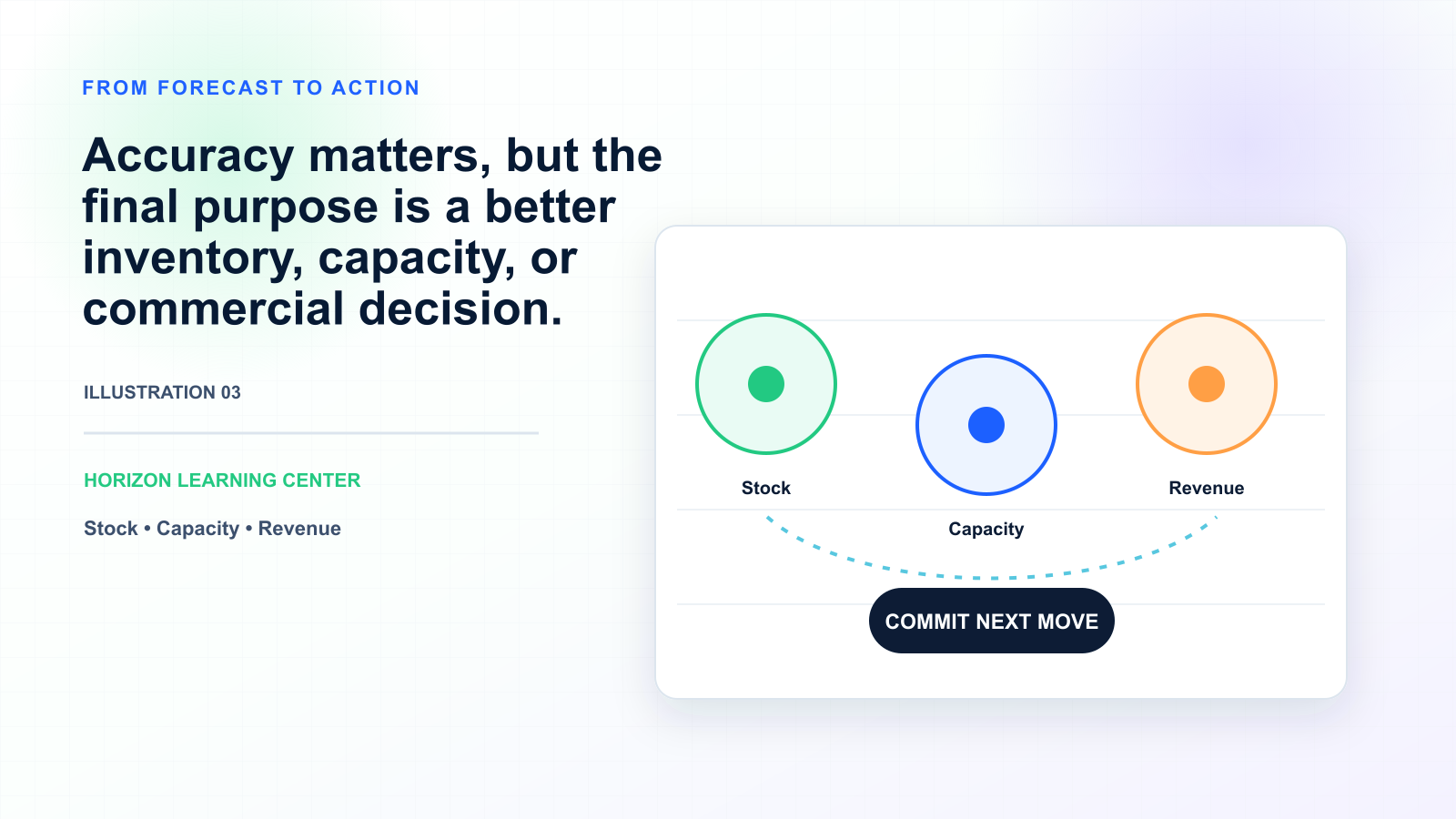
Mature demand planning requires fluency across these concepts. Platform evaluations involve them — vendors describe capability in this vocabulary. Operational discussions reference them. Improvement initiatives depend on understanding which concepts apply where. Companies whose planning teams have shallow concept fluency typically extract less value from sophisticated platforms because they can't fully use the capabilities.
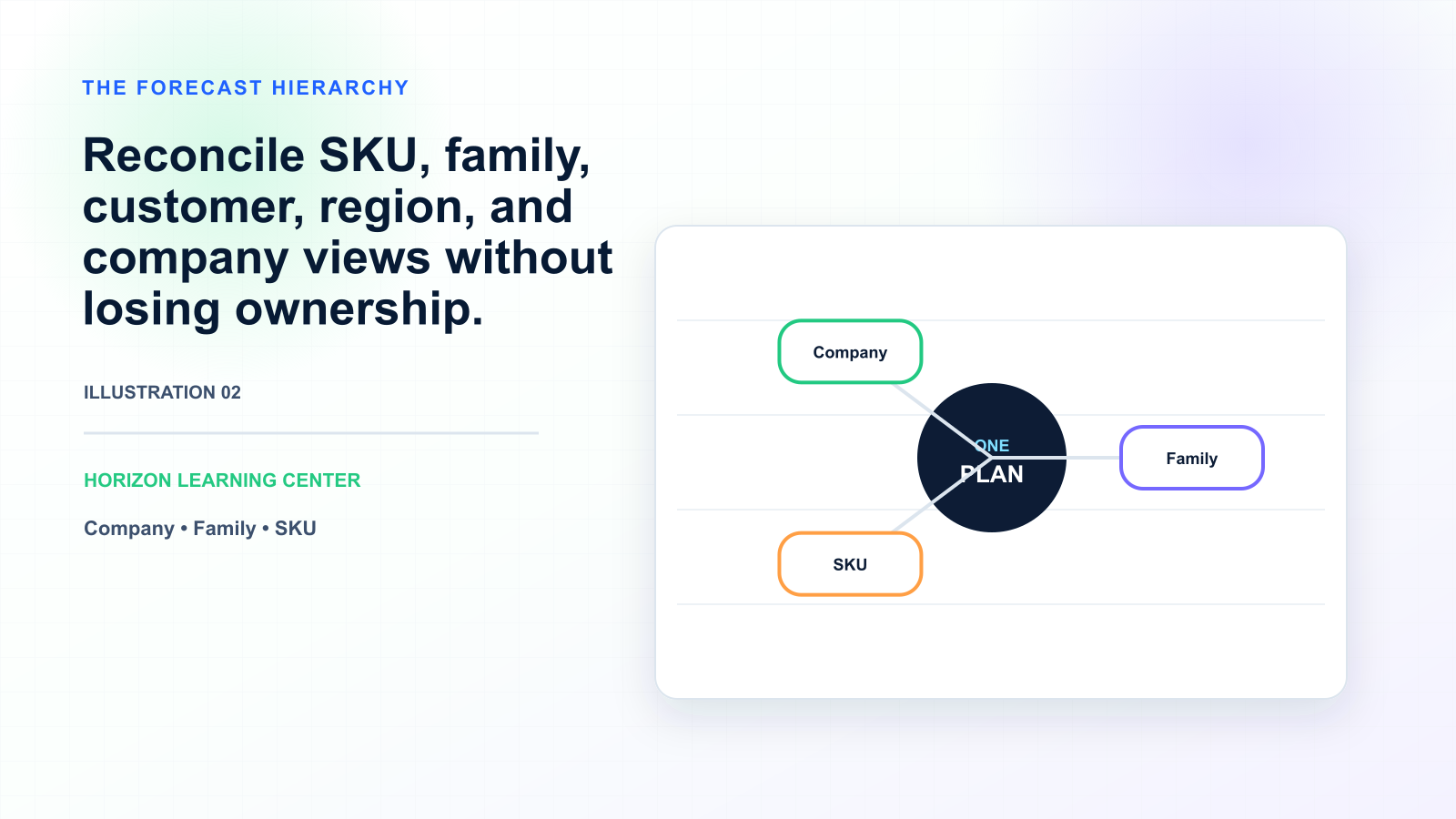
Forecast accuracy measures how closely forecasts match actuals. Multiple metrics exist because different operational questions need different measurement:
MAPE (Mean Absolute Percentage Error): Average of absolute percentage errors. Easy to understand but problematic for SKUs with low absolute values (small errors become large percentages). Formula: |Forecast - Actual| / Actual, averaged across periods or SKUs.
WMAPE (Weighted MAPE): MAPE weighted by volume or value. Gives high-value SKUs more influence on the metric. More representative of business impact than unweighted MAPE for portfolios with skewed value distribution.
MAD (Mean Absolute Deviation): Average of absolute differences (not percentages). Useful for value-weighted accuracy when measuring in dollars matters more than percentages.
RMSE (Root Mean Square Error): Penalizes large errors more heavily than small errors. Appropriate when occasional large errors matter more than consistent small errors.
The honest practical guidance: pick 1-2 primary metrics aligned with your business priority and track consistently. Companies that switch metrics frequently make accuracy improvement harder to measure.
Bias differs from accuracy. Accuracy measures total deviation (regardless of direction). Bias measures systematic directional error — are you forecasting too high or too low on average? Total accuracy can look acceptable while bias is significant.
Bias matters operationally because it doesn't average out. Consistent over-forecasting builds excess inventory. Consistent under-forecasting causes service failures. Both are costly even when MAPE looks fine.
Tracking Signal: Standard bias monitoring metric. Cumulative bias divided by mean absolute deviation. Values above +4 or below -4 typically indicate systematic bias warranting investigation. Tracking signal is a continuous monitor rather than periodic measurement.
Simple Moving Average: Average of recent N periods. Baseline method, appropriate only for very stable demand. Limited by inability to capture trend or seasonality.
Exponential Smoothing: Weights recent observations more heavily than older ones. Variants handle different patterns: simple exponential smoothing for stable demand, Holt's method for trend, Holt-Winters for trend and seasonality.
ARIMA (Autoregressive Integrated Moving Average): More flexible time-series method. Captures complex autocorrelation patterns. SARIMA adds seasonal components. Requires more data and computational complexity than exponential smoothing.
Croston's Method: Designed for intermittent demand (slow-moving SKUs with sporadic orders). Separates demand into magnitude and inter-arrival time, forecasting each separately. Standard methods systematically over-forecast intermittent demand; Croston handles it appropriately.
Syntetos-Boylan-Approximation (SBA): Refinement of Croston's method addressing certain biases. Used for intermittent demand alongside or instead of Croston.
Gradient Boosting (XGBoost, LightGBM): Ensemble of decision trees that learn from residuals iteratively. Strong for incorporating multiple input features (price, promotion, weather, calendar). Requires sufficient training data and feature engineering.
Random Forests: Ensemble of decision trees with random feature selection. Less prone to overfitting than single trees. Useful but typically less accurate than gradient boosting for forecasting.
Neural Networks: Deep learning methods including LSTM (Long Short-Term Memory) for time series. Strong for complex non-linear patterns and long-term dependencies. Requires substantial data and computational resources.
Prophet: Facebook's open-source time series method. Handles trend, seasonality, holiday effects, and missing data well. Often produces reasonable forecasts with limited tuning, making it popular for general use.
Causal methods incorporate external factors (price, promotional activity, weather, economic indicators) into forecasting. Regression-based causal forecasting fits coefficients to observed historical relationships. ML-based causal methods can capture non-linear relationships. Causal methods deliver substantial accuracy gains when relevant factors are clean and available, but require data infrastructure to capture causal factors properly.
Ensemble methods combine multiple methods, selecting the best per SKU automatically. Modern ensemble approaches typically include 8-20 methods across statistical and ML categories. The selection logic uses holdout accuracy with stability checks to avoid selecting methods that look great on one period but vary widely. See How Ensemble Forecasting Works for detailed treatment.
Forecast horizon is how far into the future forecasts extend. Different horizons serve different decisions:
Short horizon (1-4 weeks): Drives execution decisions — fulfillment, inventory transfers, expediting. Forecast accuracy at this horizon affects daily operational decisions.
Medium horizon (1-3 months): Drives supply planning — production scheduling, supplier orders, capacity allocation. Most operational supply chain decisions happen at this horizon.
Long horizon (3-18 months): Drives capacity decisions — capital investment, headcount planning, supplier capacity commitments. Forecasts at this horizon support strategic decisions.
Strategic horizon (18+ months): Drives strategic decisions — market expansion, product portfolio, network design. Long-term forecasts often shift from quantitative to scenario-based.
The practical insight: forecast accuracy expectations should differ by horizon. Long-horizon forecasts are inherently less accurate than short-horizon. Optimizing accuracy at horizons that don't match decision horizons wastes analytical effort.
Forecast lag is the time gap between when a forecast is made and when the forecasted period occurs. A forecast made in January for May has 4-month lag. Forecast accuracy typically declines with lag length because uncertainty accumulates over time.
Measuring accuracy by lag matters operationally because supply chain decisions happen at specific lags. If supplier lead times are 8 weeks, the 8-week-lag forecast is what supply decisions use — measuring overall accuracy without breaking out by lag obscures the operational reality.
Demand sensing uses short-cycle data (point-of-sale, recent orders, market signals) to refine near-term forecasts. The methodology: incorporate the latest available information to adjust forecasts faster than monthly statistical model refresh would.
Demand sensing delivers most value for: retail-heavy CPG with point-of-sale data integration, fast-cycle products with rapid demand pattern changes, promotional planning where short-cycle market signals matter, B2B operations with significant customer order rate variability.
Limited value for: slow-moving items where short-cycle signals are too sparse, B2B with monthly batch order patterns, deep capital equipment with long demand cycles, products without external data sources to sense from.
FVA measures whether each step in the forecasting process adds or subtracts accuracy. The standard analysis: compare accuracy at each step (statistical baseline, ML overlay, planner adjustment, S&OP consensus, executive override) to baseline accuracy. Steps adding accuracy have positive FVA; steps subtracting accuracy have negative FVA.
The common finding: planner overlays add positive FVA for some SKUs and patterns and negative FVA for others. The discipline becomes selectively overlaying only where overlays add value. This typically improves both forecast accuracy and planner productivity (less time spent on overlays that don't help).
Outliers are historical data points that don't represent normal demand patterns: one-time large orders, system errors, demand spikes from specific events that won't repeat. Without handling, outliers skew forecasting models and produce systematically wrong forecasts going forward.
Detection: statistical methods (values beyond N standard deviations from mean, isolated peaks in time series) identify candidate outliers. Treatment: replace outlier values with normalized values, tag periods as one-time events excluded from model training, or apply causal explanation if the outlier source is known. The honest qualifier: poorly handled outliers cause more forecast accuracy problems than most other issues — and outlier handling is often under-invested.
Repeated patterns within a year. Examples: summer cooling product demand, winter heating, holiday retail surges, agricultural cycles. Modeled in seasonal forecasting methods (Holt-Winters seasonal, SARIMA, Prophet's seasonality components).
Underlying directional movement over time. Growth (positive trend), decline (negative trend), or stability. Distinguished from seasonality (cyclical) and random variability.
Additional demand driven by promotional activity beyond baseline. Modeled separately from baseline demand because mixing them in standard models degrades both. Requires structured promotional history tagging in source data.
NPI forecasts products without history. Standard time-series methods can't forecast without data. NPI approaches include:
Analog-based methods: Find similar products (similar pricing, similar category, similar launch context) and apply their patterns. Works when truly similar analogs exist.
Lifecycle curve methods: Apply expected launch patterns (e.g., S-curve adoption) with adjustments for specific market context.
Structured judgment: Frameworks for planner input incorporating market intelligence, expected adoption rates, competitive positioning, marketing support.
The honest qualifier: NPI forecasting is inherently uncertain. The gap between best-practice NPI forecasting and unstructured approaches is significant, but no method makes NPI as accurate as established product forecasting.
EOL forecasts demand for products being phased out. Approaches include: declining trend models with explicit end-date constraints, customer notification effect modeling (announcing EOL affects demand patterns), substitution modeling (demand transfer to replacement products), run-out planning to manage final inventory levels.