Companies running multi-location operations almost always face inventory imbalance — too much in some locations, too little in others, despite (theoretically) similar demand patterns and service levels. The symptoms are familiar: stockouts in some locations while other locations have months of supply, frequent inter-location transfers, working capital tied up in slow-moving stock in one warehouse while another stockouts of the same SKU.
The honest framing: inventory imbalance is rarely a problem that can be solved by better inventory math alone. It's a symptom of underlying issues — forecast accuracy by location, lead time variability handling, service level segmentation, or distribution network design. This guide covers practical diagnostic approaches and the underlying fixes.
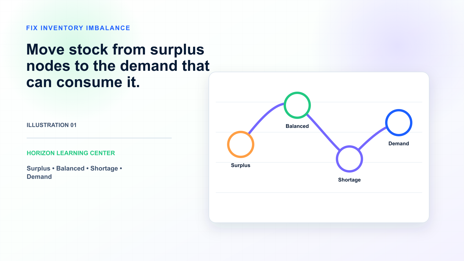
Horizon supports inventory imbalance resolution through: multi-echelon inventory optimization (MEIO) for networks with multiple locations, location-specific forecasting with ensemble methods and per-SKU model selection, lead time variability handling that flows from supplier performance into safety stock calculations, segmented service level capability by SKU class and location, proactive transfer planning recommendations through the decision execution layer.
The honest qualifier: imbalance resolution is often more diagnostic than algorithmic. Understanding why imbalance exists matters more than running better math on the same flawed inputs. Horizon supports both — better math (MEIO, stochastic safety stock) and better diagnostics (imbalance metrics, per-location accuracy tracking).
Inventory imbalance is expensive in two ways. Direct cost: excess inventory in some locations represents working capital that could be deployed elsewhere, plus carrying cost (storage, insurance, obsolescence risk). Indirect cost: stockouts in other locations damage service levels, force expensive inter-location transfers, and sometimes drive lost sales. The total cost typically exceeds what would be calculated just from excess inventory at one location plus stockout cost at another — the systemic inefficiency compounds.
What's important: total system inventory can look fine while imbalance is severe. Looking only at company-level inventory metrics misses the imbalance issue entirely.
The first step is measuring imbalance, not just inventory. Standard metrics: days of supply by location by SKU, weeks of cover variance across locations for the same SKU, stockouts by location, inter-location transfer frequency and volume. The metrics should show which SKUs in which locations have what imbalance pattern. Companies that only track total inventory or aggregate days of supply miss the imbalance entirely.
Imbalance typically traces to one or more of these causes. Forecast accuracy varies by location: if forecast accuracy is much better at some locations than others, inventory builds up where forecasts over-estimate and runs short where they under-estimate. Diagnostic: measure forecast accuracy and bias by location for the same SKU. If accuracy or bias varies significantly, this is likely a primary cause.
Lead time variability handling: if some locations have higher lead time variability from upstream sources but safety stock formulas treat lead time as constant, those locations will stockout more frequently while average inventory looks fine. Diagnostic: measure actual lead time variance by location-supplier combination. Locations with high variance and inadequate safety stock typically stockout.
Service level segmentation: if all SKUs in all locations have the same service level target, some get more than they need and others get less. Diagnostic: are service level targets segmented by SKU class (A/B/C) and by location-SKU combination based on demand patterns? If not, this is a common cause.
Distribution network mismatch: if customer demand patterns shifted (customer added, customer location changed, customer ordering pattern changed) but distribution network didn't adapt, inventory positions become misaligned. Diagnostic: review whether current network design matches current customer demand patterns.
Reactive rather than planned transfers: if inter-location transfers happen reactively when stockouts occur rather than planned proactively, locations get out of balance and stay out of balance. Diagnostic: are transfers driven by planning recommendations or by emergency response?
For each cause identified, the fix is different. Forecast accuracy by location: implement location-specific forecasting models, ensure data quality by location, address per-location bias through FVA tracking and overlay discipline.
Lead time variability: replace deterministic safety stock formulas with stochastic methods that account for lead time variability. Multi-echelon inventory optimization (MEIO) handles this natively.
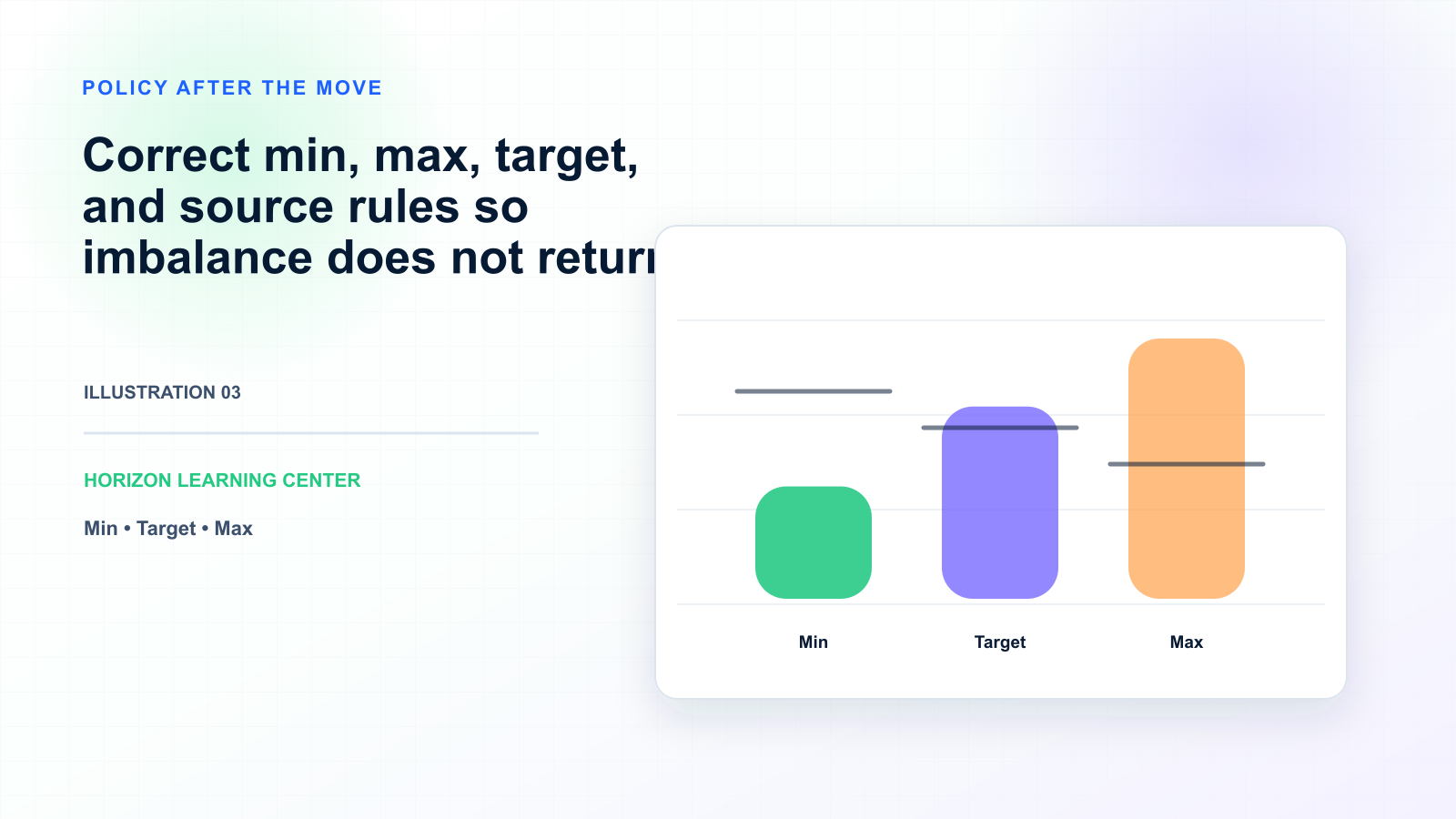
Service level segmentation: implement segmented service level targets by SKU class and location. A-class SKUs in primary distribution centers may need 98% service; C-class SKUs in secondary locations may be fine at 90%. The segmentation reduces total inventory while improving service where it matters.
Distribution network: periodically review network design against current demand patterns. This is strategic work, not weekly planning — typically done annually or after significant customer changes.
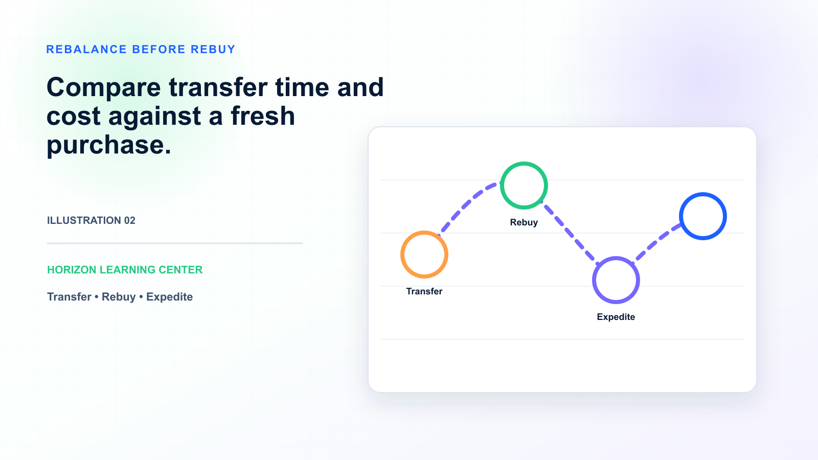
Planned transfers: implement proactive transfer planning that anticipates imbalance before it becomes acute, rather than reactive transfers responding to stockouts.
For complex multi-location operations, MEIO mathematics specifically address the imbalance problem. MEIO considers all locations together rather than each location separately, optimizing service levels and inventory positions across the network. Demand variability at distribution centers gets risk-pooled with manufacturing buffer inventory; service level targets account for inter-location transfer feasibility; inventory positions reflect the network optimum rather than per-location optimum.
MEIO capability exists in modern integrated SCP platforms (Horizon, Logility, RELEX, Kinaxis) and specialists (ToolsGroup). The math is genuinely different from single-location safety stock formulas, and the operational improvement can be substantial for networks with significant complexity.
Inventory imbalance returns when underlying conditions change — new customers, network changes, supplier shifts, demand pattern changes. Build monitoring into the regular planning rhythm: imbalance metrics in weekly inventory review, root cause investigation when imbalance reappears, structured response rather than reactive transfers.