Supply planning translates demand forecasts into feasible production and procurement plans considering capacity, materials, and lead time constraints. This guide covers the concepts that matter most for understanding modern supply planning — what they mean, how they work, when they apply, and how they interact.
The concepts are presented in approximate operational sequence — from foundational (MRP, lead time) through inventory math (safety stock, service level, MEIO) to coordination concepts (ATP, CTP, bullwhip effect).
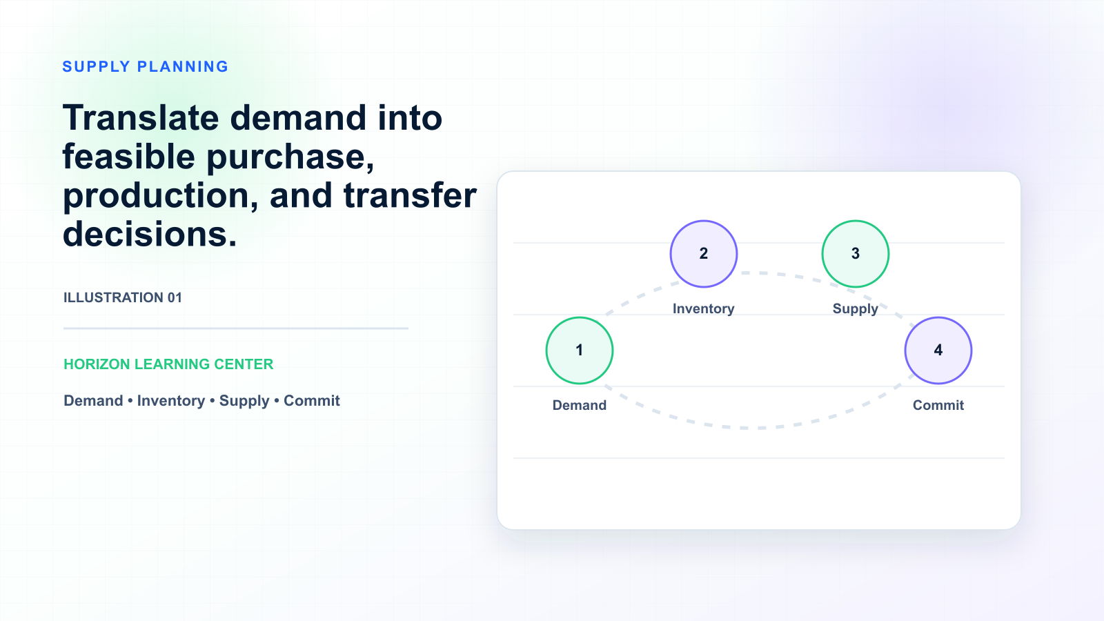
Mature supply planning applies these concepts together. Lead time and lead time variability flow into safety stock calculations. Safety stock methodology (stochastic, probabilistic for intermittent demand) drives appropriate buffer for different SKU types. Segmented service levels reallocate inventory across SKU classes. MEIO positions inventory across network echelons. ATP/CTP enables accurate customer commitments. Finite capacity planning produces executable supply plans.
Platforms vary in which concepts they implement and how well. Modern integrated platforms (Horizon, Logility, RELEX, Kinaxis, o9, SAP IBP) cover most concepts with varying depth. ERP-based MRP typically covers basic concepts but lacks stochastic safety stock, MEIO, and sophisticated ATP/CTP. The choice of platform should match the concepts most important to operational reality.
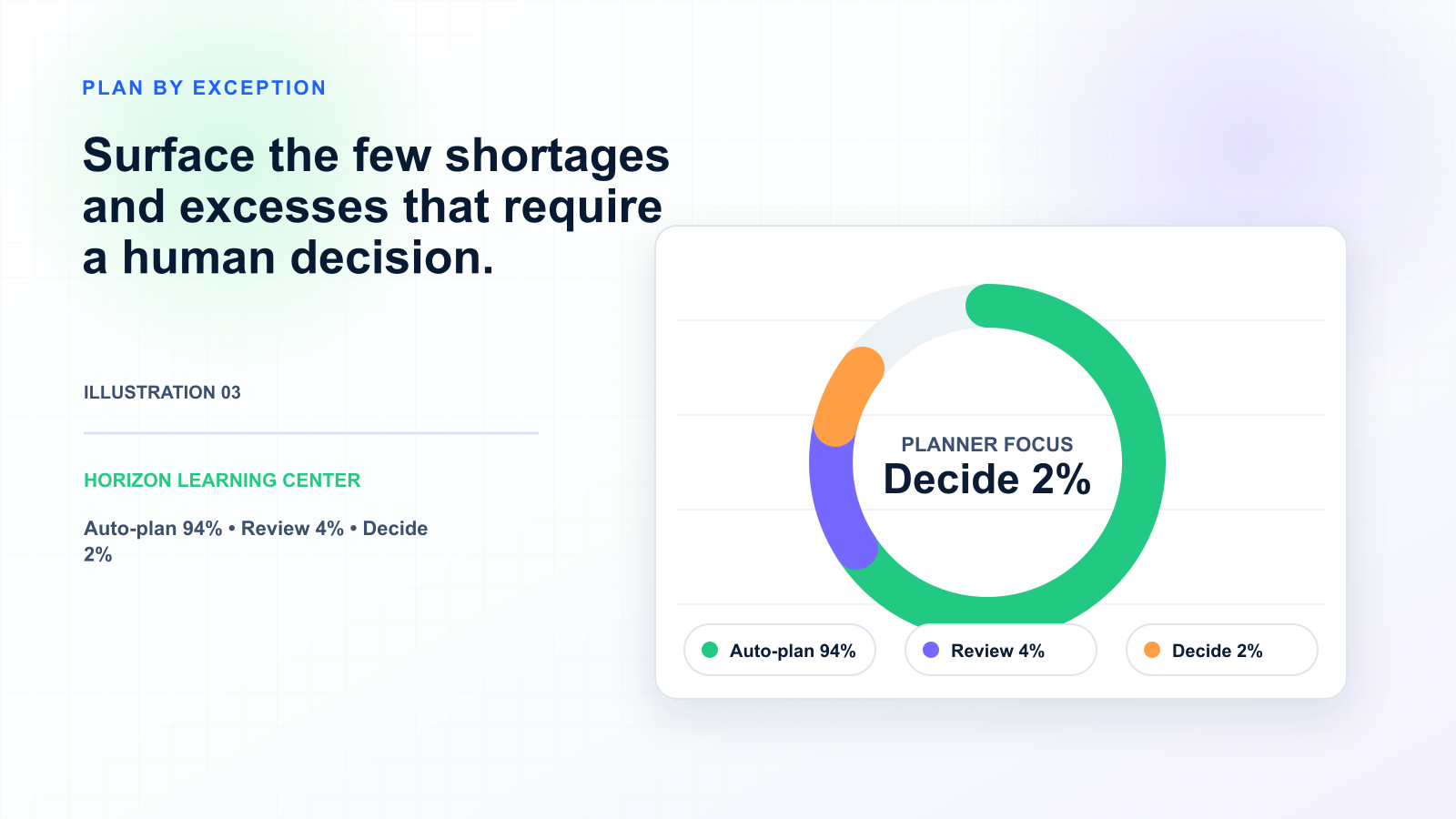
Supply planning effectiveness depends on understanding these concepts. Platform evaluations involve them. Operational decisions depend on them. Inventory and capacity decisions live or die based on which concepts are applied correctly. The gap between mature supply planning practice and basic MRP-driven planning often traces to which of these concepts are applied operationally.
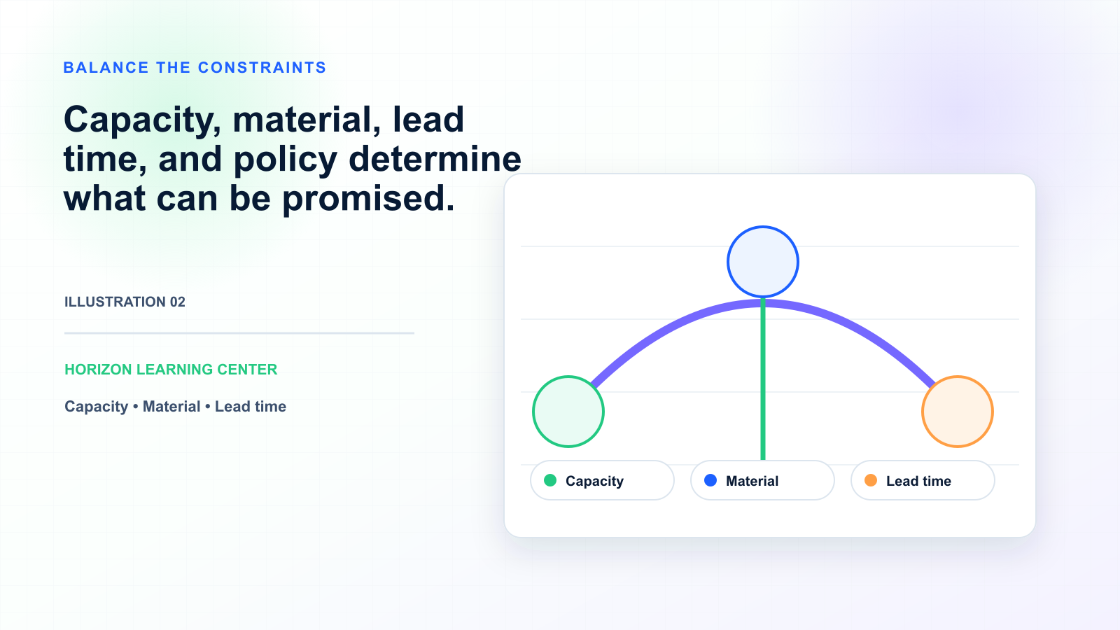
MRP calculates material requirements based on demand, bill of materials (BOM), and current inventory positions. The logic: explode end-item demand through BOMs to component demand, net against on-hand inventory, generate replenishment recommendations sized to lead times. MRP has been the foundation of manufacturing planning since the 1960s.
Traditional MRP makes simplifying assumptions: infinite capacity (calculates what's needed without checking capacity feasibility), constant lead times (treats supplier lead times as fixed parameters), deterministic demand (uses point forecasts without uncertainty handling), independent SKUs (doesn't optimize across SKUs jointly). These assumptions often don't match operational reality, which is why MRP outputs typically require human review and adjustment before becoming executable plans.
Advanced Planning and Scheduling (APS) extends MRP by handling capacity constraints, lead time variability, and sometimes optimization across SKUs. The transition from MRP-only to APS-enhanced planning is one of the most common supply chain capability upgrades.
Lead time is the time from order placement to receipt. Components: supplier production lead time, transportation time, receiving and quality inspection time, putaway time. Total lead time is the sum, but variability can occur in any component.
Quoted lead time and actual lead time often differ significantly. Variability sources: supplier production variability, transportation delays, customs and regulatory processing, quality issues requiring rework. Standard supply planning treats lead time as constant — which is often wrong. Companies measuring actual versus quoted lead time typically discover substantial variability they hadn't accounted for.
Safety stock calculations need to incorporate lead time variability for accuracy. The standard formula Safety Stock = Z × σ × √L assumes constant L (lead time). The corrected formula incorporates lead time variability: Safety Stock = Z × √(L × σD² + D² × σL²) where σD is demand variability and σL is lead time variability. The corrected formula often produces substantially higher safety stock for SKUs with significant lead time variability — appropriately so, since the standard formula systematically under-provisions these SKUs.
Safety stock is inventory held above expected demand to buffer against forecast error and supply variability. The purpose: maintain target service levels in the face of uncertainty. Without safety stock, any forecast error or supply delay would create stockouts.
Deterministic methods: Standard formulas using normal distribution assumption, constant lead time, demand and lead time independence. Simple to calculate but make assumptions that are often wrong. Typically produce safety stock that's too high for some SKUs and too low for others.
Stochastic methods: Handle non-normal demand distributions, lead time variability, demand-supply correlation. More accurate but more complex calculation. Modern platforms compute stochastic safety stock natively; Excel implementations are possible but require significant effort.
Probabilistic methods for intermittent demand: Croston-derived approaches, Bayesian methods for SKUs with sporadic order patterns. Standard safety stock approaches systematically over-provision intermittent demand SKUs; probabilistic methods correct this.
Setting service levels by SKU class (A/B/C) and possibly customer or location segment. The math: A-class SKUs (top 20% by revenue or criticality) at 98-99%, B-class at 94-96%, C-class at 88-92%. The segmentation reallocates inventory to where it matters most — reducing total inventory while improving service on important SKUs.
MEIO optimizes inventory across all locations in a network together, rather than each location independently. Considers: manufacturing buffer stock, regional distribution centers, satellite warehouses, inter-location transfer feasibility. The result: total network inventory positioned optimally across echelons.
Single-location safety stock calculations optimize per-location but ignore network dynamics. Demand variability at distribution centers can pool with manufacturing buffer (risk pooling). Service levels can be met through transfers rather than per-location safety stock. Network-level optimum differs from sum of per-location optima.
Typical MEIO benefit: 10-20% network inventory reduction while maintaining or improving service. Larger benefits for complex networks (more locations, more SKU-location combinations); smaller benefits for simple networks (few locations).
MEIO requires specific platform capability. Native MEIO is available in: integrated SCP platforms (Horizon, Logility, RELEX, Kinaxis, o9, SAP IBP) and specialists (ToolsGroup). Basic MRP platforms typically don't include MEIO. The capability gap matters for multi-location operations.
Service level is the target probability of meeting demand from stock without stockout. Common definitions vary: fill rate (percentage of orders or units shipped from stock), order fill rate (percentage of complete orders shipped from stock), cycle service level (probability of not stocking out during a replenishment cycle).
Higher service levels require more inventory. The relationship is non-linear: moving from 95% to 98% requires substantially more safety stock than moving from 90% to 93%. Moving from 98% to 99% requires substantially more again. The implication: setting service levels uniformly high across all SKUs ties up substantial working capital with diminishing returns.
Inventory level triggering a replenishment order. Calculation: ROP = (Average Demand × Lead Time) + Safety Stock. When current inventory falls to ROP, place a replenishment order sized for next cycle plus safety stock buffer.
Order quantity minimizing total cost of ordering plus carrying cost. Formula: EOQ = √(2DS/H) where D is annual demand, S is order cost, H is annual carrying cost per unit. Theoretical foundation more than operational practice in modern supply chains — most modern operations don't optimize order quantities through EOQ because the assumptions (constant demand, constant lead time, no quantity discounts) don't match reality.
Determining order quantities given operational constraints. Common approaches: fixed order quantity (always order same amount), period order quantity (order enough for fixed period), least unit cost (consider quantity discounts), least total cost (minimize total cost including carrying), lot-for-lot (order exactly what's needed). Selection depends on operational economics and constraints.
ATP is available inventory plus scheduled receipts not yet committed to existing orders. Used to commit delivery dates to new customer orders. The logic: check ATP at the required date; if sufficient, commit; if insufficient, propose alternative dates or quantities.
CTP extends ATP to include production capacity availability. Used when current inventory and scheduled receipts can't meet demand but additional production is feasible. The logic: check if capacity can produce the requested quantity by the required date; if yes, commit and create production order; if no, propose alternatives.
Modern e-commerce and customer service expectations require accurate, real-time order commitments. ATP/CTP capability enables this. Platforms without robust ATP/CTP often struggle with order commitment accuracy, leading to either over-promising (and missing dates) or over-conservative promising (and losing orders to competitors).
Amplification of demand variability moving upstream through supply chain. Retailer sees moderate demand variability; distributor sees larger variability in orders from retailers; manufacturer sees even larger variability in distributor orders; suppliers see largest variability. The effect compounds and causes systematic inventory imbalances and capacity inefficiency throughout the chain.
Order batching (placing larger orders less frequently amplifies variability), demand signal interpretation (reading temporary demand changes as trends), lead time variability (longer lead times amplify variability), shortage gaming (over-ordering when shortages expected), price fluctuations (forward-buying during promotions). Each cause is addressable but rarely fully eliminated.
Information sharing (visibility across supply chain reduces demand signal misinterpretation), smaller order batches (reduces batching contribution), stable lead times (reduces variability amplification), demand smoothing through promotional planning, supplier collaboration on capacity and lead time commitments. Modern integrated SCP platforms support several of these mitigations through visibility and collaboration features.
Traditional MRP assumes infinite capacity — calculates what's needed without checking whether capacity can produce it. Produces "plans" that may not be executable as-is. Requires human capacity reconciliation to convert to feasible plans.
Advanced Planning and Scheduling respects actual capacity constraints. Calculates feasible plans within capacity limits, identifying capacity gaps where demand exceeds capacity. The improvement: outputs are typically executable without major modification, freeing planner time for higher-value work.
The shift from infinite-capacity MRP to finite-capacity APS is one of the most common supply chain capability upgrades. The benefit: more reliable plans, less manual reconciliation work, better capacity decision support. The cost: APS systems are more complex and require more configuration than basic MRP.